
Physics 2212, Sim 12: Inductance and RL Circuits
Eric Murray, Summer 2020
Required Advance Reading
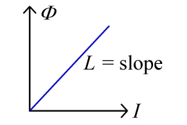 Inductance is the ratio of the magnetic flux in an inductor, Φ, to the current through the inductor, I.
L = Φ/I
Unfortunately, the magnetic flux is difficult to measure.
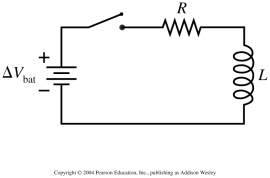 When a constant electric potential difference is suddenly applied across a circuit consisting of an inductor and a resistor in series, the potential difference across the inductor, ΔVL, the potential difference across the resistor, ΔVR, and the current in the circuit, I, all vary with time, t. There is a characteristic time, τ, called the time constant. For example, the potential across the inductor varies with time according to
ΔVL = ΔVL0e-t/τ
where ΔVL0 is the potential difference across the inductor at time t = 0, the instant the switch is closed.
To determine τ, you will fit a function of the potential difference across the inductor vs. time graph to a linear curve,
-ln(ΔVL/ΔVL0) = Bt
where B is the slope of the fit line and is related to the time constant by τ = 1/B. The inductance of the inductor can be calculated as τ = L/R.
Error Analysis
Using linear regression to fit the line will provide not only the fit parameter B, but also its experimental uncertainty, ΔB. Finding the time constant from the fit parameter using τ = 1/B is straightforward, but Δτ is not ΔB. (For one thing, Δτ and ΔB have different units.)
If we had multiple measurements of τ, we could calculate an average and standard error, and report the standard error as the experimental uncertainty in the average. On the other hand, sometimes it is necessary to calculate an experimental uncertainty from the uncertainty in one or more measured parameters.
In general, if a calculated result y is a function of measured parameters x1, x2, …, xn, each of which has an uncertainty Δx1, Δx2, …, Δxn, then the uncertainty in y can be calculated by
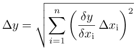
where δy/δxi is the partial derivative of y with respect to xi. (Partial derivatives, if you have not encountered them, are even easier to find than regular
derivatives, because you pretend that everything, other than the parameter you are taking the derivative with respect to, in this case xi, is a constant.) This is the error propagation
formula, and it is assumed that the uncertainties in all the measured parameters xi are independent.
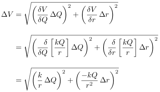
Consider, for example, calculating the electric potential due to a point charge from measured values of Q ± ΔQ and r ± Δr. The potential with respect to zero at infinity would be found using V = kQ/r. The uncertainty in V (not to be confused with a potential difference despite being expressed as ΔV) is
You should now be able to find the relationship between the uncertainty in the time constant, Δτ, and the uncertainty in the fit parameter, ΔB.
As L is proportional to B, the uncertainty in L is proportional to the uncertainty in B.