Physics 2212, Lab 8: Capacitance and RC Circuits
Eric Murray, Fall 2006
Question these experiments will enable you to answer: Is the capacitance of your capacitor within the manufacturer's tolerance? What is the time constant of your RC circuit?
Features: First, the circuit element investigated is a capacitor. Devices that are interfaced to a computer automate both the application of a potential difference, and the measurement of the resulting current. Charge is calculated as the area under the current vs. time graph. Capacitance is calculated as the slope of a charge vs. potential difference plot.
 Next, a series RC circuit is investigated. As a potential difference is applied or removed across the circuit, the potential difference across the capacitor, the potential difference across the resistor, and the current through the circuit, decay exponentially with time. Fitting a general exponential decay curve to the appropriate portions of the graphs enables the time constant of the circuit to be calculated.
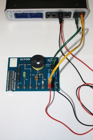
Preliminaries: Build the 100 µF capacitor circuit. The potential difference is supplied by the "output" sockets, and measured by a voltage sensor
in analog channel A. (The supplied current will be measured by the PASCO interface internally.) There are many valid ways to build this circuit, but an example is illustrated (and linked to a larger image). Open the data template. You'll find a graph for the potential across the capacitor and the current provided by the PASCO interface function generator as a function of time. The function generator is set to provide a potential difference that varies with time as a 49 Hz ramp up wave having a 5.0 V amplitude. After Record
is clicked, data will be collected for 0.010 s after the potential difference rises through zero volts, thereby recording nearly one entire positive half-cycle of potential difference. Nothing need be calibrated.
Experiment 1: Click Record
. Data will be collected for 0.010 s. Record the potential difference across your capacitor and the charge on your capacitor at 1.0 ms intervals. The potential difference is easiest to find with the cross-hairs on the potential vs. time graph. You may need to change the properties of the cursor tool to show more decimal places. The charge on the capacitor is the integral of the current to it over time, and can be found by selecting the appropriate region of the current vs. time graph (zero to 1.0 ms, for example) and determining the area under the curve with the area tool.
Graph the charge on your capacitor as a function of potential difference. Find the capacitance (slope of the graph) with its standard error. An Excel spreadsheet is recommended. Note that capacitors are often manufactured with a tolerance of ±20%.
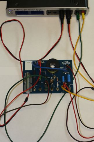
Experiment 2: Build a series RC circuit using your (nominally) 100 µF capacitor and a 100 Ω resistor. You may measure the resistance of your resistor using your DMM. There are many valid ways to build this circuit, but an example is illustrated (and linked to a larger image). Predict the time constant for your circuit, and record your prediction.
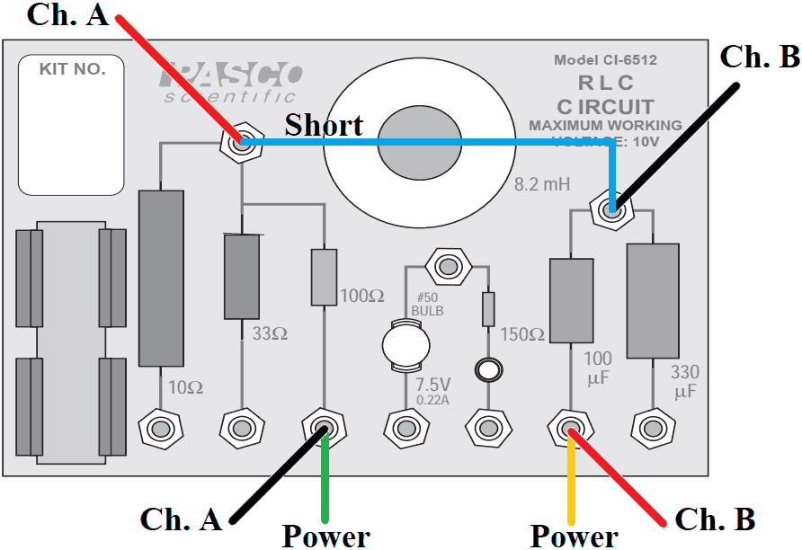
 The potential difference across the resistor is measured by a
 voltage sensor
in analog channel A. The potential difference across the capacitor is measured by a voltage sensor
in analog channel B. The supplied current will be measured by the PASCO interface internally. Open the data template. You'll find a graph for the potentials across the resistor and capacitor, and the current provided by the PASCO interface function generator, as a function of time. The function generator is set to provide a potential difference that varies with time as a 10 Hz positive square wave having a 5.0 V amplitude. Data will be collected for 0.20 s after Record
is clicked, thereby capturing several cycles. Nothing need be calibrated.
Click Record
. Once data collection is complete, select a region on the current vs. time graph that shows a complete decay half-cycle (i.e., current is positive and decreasing). Select a Natural Exponential
from the fit menu. Record the fit parameter B and its uncertainty ΔB. Calculate the time constant and its uncertainty.
Fit a Natural Exponential
curve to appropriate regions of the capacitor potential vs. time graph, and the resistor potential vs. time graph. Find the time constant and the uncertainty of each, as you did with the current. How do the three time constants compare to the value you predicted?
Summary: Review your worksheet. Think about the goals of these experiments, your results, and the expectations from theory while writing your discussion.
 Next, a series RC circuit is investigated. As a potential difference is applied or removed across the circuit, the potential difference across the capacitor, the potential difference across the resistor, and the current through the circuit, decay exponentially with time. Fitting a general exponential decay curve to the appropriate portions of the graphs enables the time constant of the circuit to be calculated.
