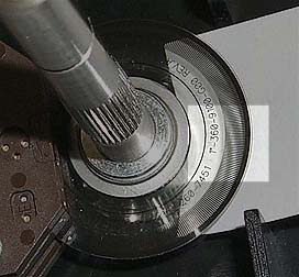
 The internal disk of the rotary motion sensor. The disk has alternating dark lines and clear spaces. A photosensor detects the frequency at which the dark lines go past the detector. |
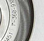 A close up of the dark lines. |
Note that software notes refer to ScienceWorkshop, not DataStudio. The DataStudio Manual is available as a PDF file.
The motion sensor is an ultra-sonic range finder. It emits a pulse of sound in a given direction and then senses the return echo from some object. The times at which the pulse is emitted and received are recorded, and the distance to the object is calculated as half the elapsed time multiplied by the speed of sound. An initial calibration is provided (effectively measuring the speed of sound) but the speed varies very little as long as the temperature is reasonably uniform. The motion sensor can make up to 50 position measurements per second and the trigger rate can be set when the calibration option is selected. For many purposes, the measurements are effectively continuous. However, when using the position data to produce graphs of velocity or acceleration, the rate should not be set too high. Velocity calculations involve dividing by the time between measurements, and any jitter in the position measurements is proportionally expanded. For the acceleration calculation, this expansion is squared!
The rotary motion sensor is a wheel whose rotation angle is accurately measured at a
series of small time intervals. The wheel may be coupled to a rotating object to record
its orientation as a function of time. Also, by running a string over the wheel and
connecting the string to an object moving in a straight line, the position of the object
may be recorded as a function of time. Using a string in this way is not always ideal
since the other end of the string must be kept taught, often by weighting it. However, the
accuracy of the rotary motion sensor is significantly better than that of other equipment
available. Several options are available for linear motion conversion; that used most
often is the intermediate pulley (groove)
.
The internal disk of the rotary motion sensor. The disk has alternating dark lines and clear spaces. A photosensor detects the frequency at which the dark lines go past the detector. |
A close up of the dark lines. |
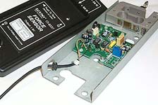
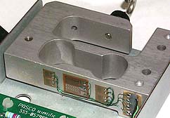
The force sensor measures the force applied to it. It may be mounted on a cart. When
selecting the force sensor, it is necessary to calibrate it (in the orientation in which
it will be used). Before making any measurements, the tare
button on the force
sensor should be pressed. Then two force measurements should be made, close to the ends of
the expected range of forces. Often, one of these is the zero force and the other is made
by attaching a string attached to a known weight to the force sensor (with the string over
a pulley if the force sensor is horizontal).
 |
 |
 |
When any device is attached to the interface box, this information must be provided to the computer software so that it can interpret the signals from the interface appropriately. The fist step is to click on either the digital plug or the analog plug and drag it to the equivalent slot on the interface box display (see diagram). This invokes a menu of possible devices; select the correct one by clicking on it. This in turn may invoke a calibration/settings option. Use this (or bypass it) as necessary. The device symbol appears below the slots on the interface box display.
Once a device has been selected by the mimicking process, a graph may be associated with the device. Click on the graph symbol and drag it to the device symbol. A menu appears so that the required variable(s) may be chosen (see Technical Note 8 for information on multiple graphs). Then the graph appears. To adjust the axis scales, click in the axis caption area and follow the instructions.
When setting up a graph, more than one measured (or derived) quantity may be selected. Then a set of graphs appears, one for each quantity, and all with the same time scale. If the graph has already been set up, click on the multiple graphs symbol (see diagram) and select the extra graph quantities. After a graph has been created, extra graphs may be added using the add graph button. Note that separate, individual graphs may be invoked by repeating the graph setup process (see Technical Note 5).
Once a device has been selected by the mimicking process, a table may be associated with the device. Click on the table symbol and drag it to the device symbol. A menu appears so that the required variable(s) may be chosen (see Technical Note 8 for information on multiple tables). Then the table appears. Usually, only the measured quantity is tabulated so, to get times as well, click on the clock symbol. To adjust the number of digits, click on the digits indicator at the top of the column and follow the instructions.
When setting up a table, more than one measured (or derived) quantity may be selected. Then a set of columns appears, one for each quantity. If the table has already been set up, click on the add column symbol (see diagram) and select the extra quantities. Note that separate, individual tables may be invoked by repeating the table setup process (see Technical Note 7).
To reduce/expand a window, such as the experiment
window, click on the
middle of the three boxes in the top right corner of the window. To move a window, click
on the top bar and drag the window so that the top left corner is at the desired location.
To resize a window, click on the bottom right corner and drag it to the desired location.
By reducing the experiment window and reorganizing the graph and/or table windows, all the
information may be displayed simultaneously. Alternatively, the graph and table windows
may be superimposed so that part of the graph extends horizontally beyond the table window
and part of the table window extends vertically beyond the graph window. Then it is easy
to switch between the windows by clicking on them alternately and, at the same time,
obtain the maximum definition and information.
The experiment window has four buttons in the top left corner, and an options button below (see diagram). The record button starts measuring and recording a new set of the measured quantities. The pause button turns recording off, temporarily, and then back on. The stop button finishes the measured set. The monitor button displays the measured values without recording them. The options button may be used to override the record and stop buttons by specifying alternate start and stop conditions. In particular, the recording of the measured quantities may be set to run for a fixed time. Click on the options button and follow instructions. The options button may also be used to add data via the keyboard. Click on the keyboard button and follow instructions.
To find the values associated with a point on a graph, click on the cross-hairs symbol in the graph window and move the arrow to the desired point. Approximate values for the point appear in the axis caption areas. More accurate values may be obtained by invoking a table (see Technical Note 3).
By moving the arrow to the top left hand corner of a desired region on a graph and dragging to the desired bottom right corner, a region may be outlined and the points in the outline selected. This allows the other points to be discounted. The same process may be applied to the cells in a table.
Once a set of data has been selected, the statistics option may be invoked by clicking on the summation symbol in the graph or table. A menu of options appears and the desired statistic may be selected (sometimes using sub-menus). Mean, standard deviation, and a linear fit are typical statistics.
The PASCO system has a built in oscilloscope display feature. To access
it drag the Scope
icon to one of the channels you wish to monitor. You
get a scope face and control panel; see Fig. 1.
 |
To the right of the display are the three "scope" channels Top controls the green trace, second is the blue and the bottom is the red trace. If you initiated the "scope" function on (say) channel A then the upper (green) display already shows A in the square box. The red and blue display boxes show an international symbol for stop (which means there are no signals and they are turned off). If you wish to display some other signal on say the red display then click on the stop sign for the red display and get a further display which allows you to choose what to put here (e.g. display channel B). You need to decide on the setting of the display amplifiers; the default value is 5V/divn which means that a 5V signal will give you only a 1 divison deflection on the screen. If your signal is expected to be (say) 0.5 volts then you will hardly see anything. For this sized signal you might want to choose 0.1 volts/divn so that the 0.5 volts signal should create a deflection of 5 divisions (5 cm).
Underneath the display is the setting of the "time base" or time sweep. The default value is 10msec/divn meaning that each division on the scale in the x-direction will correspond to 10 milliseconds or 10-2 second. Again you need to start off by choosing a value which is appropriate to the thing you wish to display. If you expect a signal which is going to oscillate one every 1/100 th of a second (i.e. a frequency of 100 Hz) then with the default setting only one oscillation will be displayed in one scale division or one cm. That might be a bit cramped. You might choose a setting of 1 msec/divn so that the 10 cm x-scale is covered in 10 msec so that one oscillation occurs in the full sweep of the trace from left to right.
The final decision is the setting of the "trigger". Basically you are going to tell the scop to start the trace whenever the signal going into the green channel exceeds a certain value and is either getting bigger or smaller (at your choice). First thing is that the "trigger" operates only on the signal going into the green scope channel (it does not trigger on the other channels). Therefore there must be some signal input connected to that channel and you must choose for this the signals which most usefully acts as a start for the problem you are studying (you decide!). Now the "Trig" icon must be "on" otherwise the trigger function is not operating; click on the "Trig" icon to ensure that it is darkened (it is not very dark--the intent is that when "on" it looks like a push button which is depressed). Next you MUST set a signal level at which the "trigger" is supposed to operate. To do this double click on the scope face to get the scope set up panel. There are two boxes which can set the start condition. Supose that you expect a 5 volt sinusoidal signal and you would like the trace to start when the voltage is -2 volts ans going more negative; then set -2 in the level box and decreasing in the direction box. Now exit the box and your trigger situation is set up. The gree triangular index to the left of the screen actually indicates the setting values you have chosen for the trigger. [Feel free to alter the trigger conditions to get a display which in your opinion is the most suitable for the problem at hand--you can't hurt anything. Also note that the "trigger" setting can be changed by pulling the green triangular icon with the computer mouse if you prefer.]
Generally you read things from the scope by just measuring position against the scale on the face of the scope. There is, however a more accurate built-in method. Click on the little button xy next to the time scale and now move your mouse around. You see a cross line on the scope face which is being moved by the mouse. The position of the line intersection is read on the y and x control panel displays (substituting for the sensitivity settings which you have previously chosen). You can read these off and record the position of any point on the trace.
It is possible to substitute for the time display on the x-axis one of the input voltages going in to the interface box. Click on the clock and select a channel. If you select channel A then when you start monitoring you will be displaying a x/y plot with channel A on the x-axis and the other channels (whatever you have selected) on the y axis.
The time base display gives a "sampling rate". This tells you how often the digital scope is "sampling" time. The 10 ms/divn default setting of the time base might give a sampling rate of 2000 times/sec. This means that the spot is moved stepwise across the screen once every 1/2000 second or 5 x 10⁻⁴ seconds. With the 10 msec/divn setting that means each division (10-2 seconds) with be drawn with 20 steps in the x direction ( 10-2 / 5 x 10⁻⁴ ). These steps are so close the trace will appear to be a continuous line and this is not a problem. For other conditions (particularly very small times per division) the steps can be a problem. Sampling rate is partly governed by the number of channels you have activated (you get a lower rate with more channels in use because the computer needs to spend time cycling through all the channels to check the data in each).
The "trigger" is the signal to the scope to start a trace. In some situations this trigger signal comes from an external event; that is not an option in the PASCO system. More normally the "trigger" responds to one or other of the signals being monitored by the scope. You can set it so it to start the trace when a particular signal is rising (or falling) and has become bigger than some particular value. You can set the trigger to be "zero" which means the trace will start at any time it is ready. Mostly one wishes to set it at some particular value so that a feature of the trace is positioned on the left hand side of the screen.
A scope with multiple traces can only trigger on one channel (obviously they all have to stay in synchronism so when one is started they all start). The PASCO scope triggers on the green channel signal only. So set up so that the signal you wish to use as a trigger is on the green channel.
To set the trigger conditions double click on the scope face to get the setting control. If you wished (say) to trigger the display to start when the voltage is going from +5 to zero then set +4.8 V (little below 5 V) and decreasing. If you wished to set the trigger to start the trace when the voltage is just changing from 0 to +5 volts then choose +0.1 V (a little above zero) and increasing.
It is important to note that the silver conducting ink reaches its proper conductivity after 20 minutes drying time. Plan your experiment period with this in mind.
If you are making a new picture from scratch (not just copying one of our standard pictures) then sketch the layout on a piece of scratch paper and plan how it will fit on the grid of the conducting paper. Any shapes can be used but keep them simple. Its best to construct a facsimile of your problem using lines, bars, circles etc. The "shapes" will be conducting (and therefore everywhere the same potential) and we will refer to them as "electrodes".
Draw the electrodes on the conducting paper, printed (grid) side up (life will be simpler if the numerals are the correct way up for your problem). Do the drawing on a smooth hard surface (e.g. the bench and not on the corkboard). Shake the conducting ink pen vigorously for 20 seconds (with the cap on). Remove the cap. Pressing the spring loaded tip lightly down on a piece of scrap paper while squeezing the barrel firmly this starts the ink flowing. Draw the pen slowly across the scratch paper and you should get a solid silver line. If the line is spotty then keep drawing until the ink runs smoothly. Now draw your electrodes on the black conducting paper. If a line becomes spotty then draw over it. It is very important that all parts of the electrode be properly joined together otherwise the device will not work. Now replace the cap on the pen and you will need to wait 20 minutes for the paint to reach its proper conductivity.
This supply is used in a number of experiments. Before ever connecting anything make sure the supply is OFF (the big green button is in the out position and no light on the supply are glowing) and turn both the control knobs under the meters fully anti-clockwise so everything is off and turned down. In the following figure is a picture of the front face and a short listing of control identifications.
First note that there are three connection terminals, positive, negative and ground. Normally you will connect your equipment between the positive and negative terminals. It is always a good idea to connect part of your apparatus to ground (otherwise the supply output "floats" which can give rise to problems). We suggest you connect the negative terminal to the ground terminal (use a banana plug lead).
There are two meters; one to read current out of the supply and one to read voltage provided by the supply. There are two control knobs under each meter; one is for a coarse control and the other for a fine control.
This supply operates in either a constant current mode or a constant voltage mode. If the light is on under current meter (red) then the current is being kept constant; if the light is on under the voltage meter (green) then the voltage is being kept constant.
Turn on the supply (depress the big green button). The constant current light will come on and the current meter will read zero (the supply is giving you a regulated current of zero). Turn up the voltage and then turn up the current. Both meters will read and the light will show which is being "regulated". Alter the controls to get the current or voltage you require and that the feature you wish to be kept constant has its light on. [In the electrostatics experiments where the supply produces a voltage for plotting on the conductive paper one obviously requires the voltage to be constant. The current will be very small and this meter may read zero. In the current balance experiments where a wire with a current interacts with a magnetic field then one obviously needs the current constant. In this experiment the voltage will be very small and this meter may read zero. The advantage of the regulation system is that if for some reason the load on the circuit changes (e.g. your finger touches the conducting paper in the field plot experiment and you draw a little extra current) then the supply automatically corrects for this and keeps the regulated feature constant.
Meters are used to measure current and voltage. Multimeters have multiple uses. With switching of internal circuitry they can be used to measure voltages and currents. The meters used in our labs give a digital reading and will also measure resistance. Since they use a battery for their operation they should be turned off when not in used by placing the rotating switch in the OFF position. The black connecting lead should always be connected to the "com" (common) socket.
There are two differen types of multimeter in use in our labs but their operation is (basically) the same and the main practical difference is in plugging in the leads. One meter type is by CEM and the other by BK Precision. Lean Connection as follows:
|
CEM Type:
Or |
Black Lead always in COM(mon) socket.
Red Lead (almost) always in VWmA (volt ohms milliamps) socket. Red Lead in 10A socket only if the current is expected to be very large (like Amps). |
|
BK Type:
Or
|
Black Lead always in the COM(mon) socket.
Red Lead in the VW (volt ohms) socket to measure volts and resistance. Red Lead in the mA (milliamp) socket to measure small currents. Red Lead in the 10A socket only if current is expected to be very large (like Amps). |
To measure a current you must break the circuit and connect the meter leads across the break so that the current flows through the meter. To set the meter to measure DC current rotate the single control knob to the DCA segment (or the A segment on the BK type) and select a number in that segment which corresponds roughly to the current you anticipate. A setting of DCA 200m means that the meter is set to measure a maximum of 200 milliamps. If the reading on the meter when is use is 77 then this means that the current is 77 miliamps. A meter setting of DCA 200µ means that the meter is set to measure a maximum of 200 microamps. If the reading on the meter when in use is 77 then this means that the current is 77 microamps.
To measure a voltage across a circuit component you must connect the two leads across that component. Set the control knob to the DCV section (V--on the BK type) to measure DC volts. Choose a setting in this section to correspond to approximately the voltage you expect. A setting of 20 on the DCV means the meter is set to read a maximum of 20 volts. A setting of 200m on DCV means the meter is set to read a maximum of 200 milivolts.
When measuring voltage the red lead is supposed to be connected to the positive side of a component (e.g. the positive side of a battery) and the black to the negative side. If you have connected it the wrong way round then the meter reading will have a negative sign in front of the digits. This does not harm the meter and just means you have the connections the wrong way round. If you wish you can change them. Alternatively just remember that with the negative sign this means the red connection is in fact connected to the negative side of the object and the black connection is connected to the positive side.
When measuring current the red lead is supposed to be connected to the point where current enters the meter and the black lead to the point where it exits the meter. If the reading on the meter has no sign in front of it then this means you have connected it the right way and you can determine the direction of current flow. If there is a negative sign in front of the digits it means the meter is connected up the wrong way round. You can either reverse the connections of the leads or else just remember that the red side is in fact connected to the point where the current exits (and the black to the point where it enters).
These meters can also be used to measure resistance of a resistor. Connect the leads to the object whose resistance you wish to measure and rotate the control knob to an appropriate part of the circular scale. The meter automatically provides a voltage across its two leads and measures the current which flows and calculates the resistance of the resistor.
There are other scales on this meter which will not be used in this lab.
Sometimes you will find that the reading of the meter changes in the last digit while you ar measuring something which you had expected to be constant. This is because in real circuits there are slight fluctuations in current flow and voltage due to thermal effects at connections. It is not a fault in the meter. If the meter is changing then the best you can do is to take the average value of the reading and use the variation in the reading as a measure of accuracy. For example if the meter is set to measure DCA 200 m and the reading is changing between 75.5 and 75.6 then the best you can say is that the current is 75.55 mA with an accuracy of +/- 0.05 mA.
On the figure (a modification of Fig 1 given in Lab #12) we have drawn the equipotential lines between two parallel plates and outside the plates. This is a case with a high degree of "symmetry". This case is fairly easy to calculate for the region of space between the plates and this is done in the text; it is difficult to calculate for the region outside the plates. You will be asked to work out potential and field for various points on this plot. Consider three locations.
 |
Case A. A point at the center between the plates and equal distance from each plate.
Potential. That is obviously 5 Volts (the 5 volt line goes through the center).
Field. Direction is certainly "down" (field is in direction of the force on a + charge). A field
magnitude is equal to the magnitude of the derivative of voltage with distance. Best you can do is
estimate this. If the 5 and 6 volt equipotentials are separated by say 3 mm then the field magnitude
is l/O.003 = 333 volts/meter. (You will find that the 4 and 5 volt lines are separated by the same
distance in this case so that the field "at" point A can reasonably be taken as the field on either
side of A).
Case B A point at the center between the plates but say 3 cm down from the top plate.
Potential. Maybe there is an equipotential line through it. If not either interpolate between the
adjacent lines or just stick the probe onto that point and read the result on the meter.
Field. Again direction is certainly down. Again take two nearby equipotential lines and work out a
field magnitude. In practise you will find (and could predict) that the equipotential lines are all
equal distance apart (distance between 5 and 6 V is the same as between 4 and 5) so the answer
will be the same as at the central point equidistant between the plates.
Case C A point 3 cm to the right of the right end of the bottom plate!
Potential. Again if there is no equipotential line through the point either interpolate or stick the
probe in and measure it. (It will be helpful in finding the field if you were to find the potential at
the point and then plot that equipotential in that region; e.g. if the potential is 1.7 Volts then plot
the line of 1.7 volt points in that region).
Field. More complicated here. The field direction will be perpendicular to the equipotential. Draw
the equipotential line through the point and take the direction as perpendicular to that line (and
roughly towards the negative plate). To find the field magnitude draw a few equipotential lines in
that region; say the 1.7 volt, 1.6 volt and 1.8 volt lines. Then measure the perpendicular distance between the lines, calculate the field to either side, and take the average is representing the field at
C. Obviously the closer together you draw the lines the more accurately you are determining the
field at point C.
This general set of techniques can be used at any location in any field situation. Plot the equipotential lines and, in essence, find the magnitude and direction of the gradient -dV/ds, which defines field.